How to Make a Pivot Table in Google Sheets

Introduction

You can make a Pivot Table in Google Sheets to simplify analysis of complex data. A Pivot Table allows you to compare values and also see trends and patters.

In this guide you will learn how to make a Pivot Table in Google Sheets.

How to Make a Pivot Table in Google Sheets

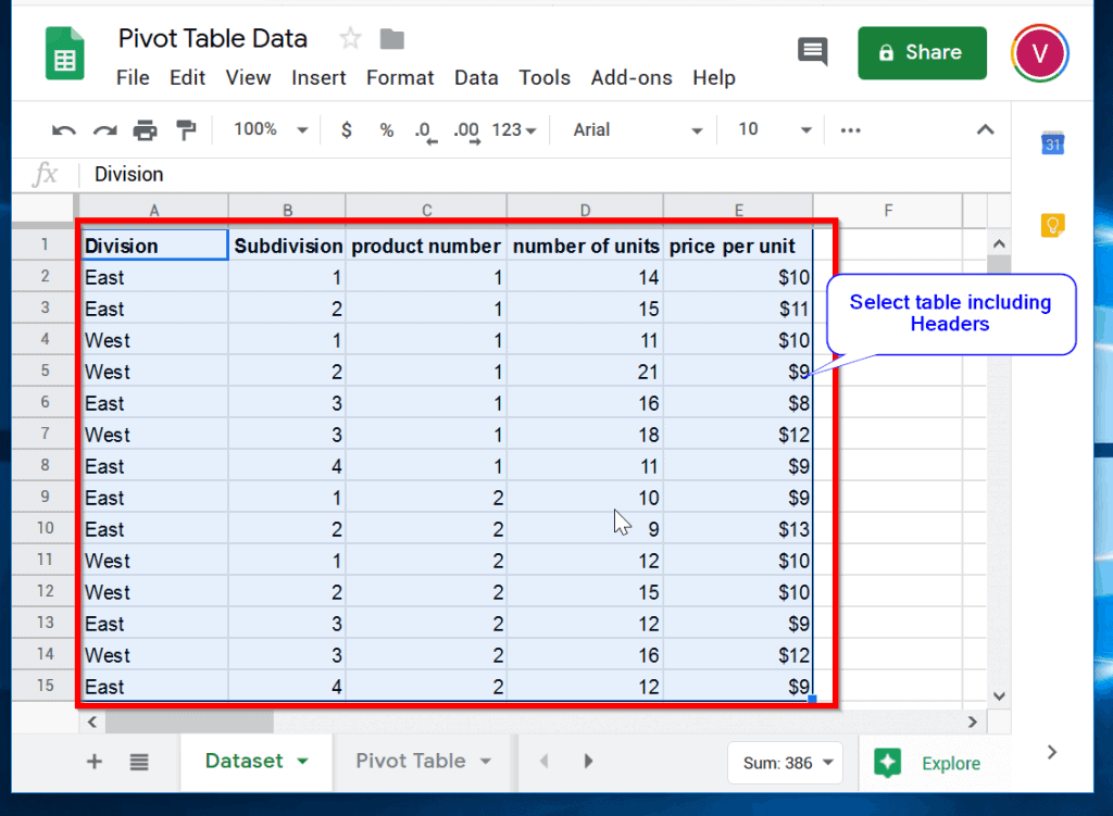
The Google Sheets table below shows sales divisions of a company, the subdivisions and information about products.

The table has a number of uncategorized data like multiple sales Divisions and Subdivisions. It also has information regarding the number of products and prices per unit.

In this example, I will show how to make a Pivot Table to sort the data by Divisions and Subdivisions. The Pivot Table will also show total number of products and Average price per unit.

To make a Pivot Table in Google Sheets, follow the steps below:

• Select the data you want to plot a Pivot Table for, including the table headers.

• Next, click Data tab.

• Then click Pivot Table. The Create pivot table option will open.

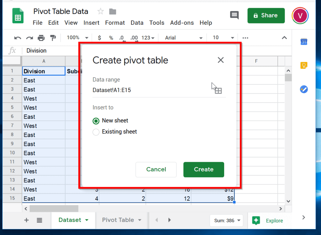
• To create a Pivot Table, click Create. This will create a blank Pivot Table as shown in the image below.

How to Add Data to a Pivot Table in Google Sheets

Once you have created a blank Pivot Table, you need to add data to the Pivot Table.

Here are the steps:

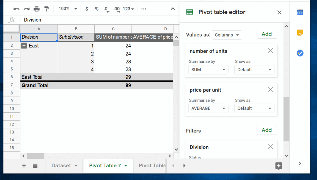
• Beside Row, click Add. Then select Divisions. Click Add again and select Subdivisions. This will add both to the Pivot Table.

• Next, beside Value As, click Add. Then select Number of units. Click Add again and select price per unit.

• To change SUM of price per unit column to average, on the price per unit section click the Summarise by drop-down. Then select AVERAGE. Leave the Show as drop-down as Default.

How to Filter Data in a Pivot Table in Google Sheets

After making a Pivot Table in Google Sheets, you may want to add some filters.

To filter the above Pivot Table by Division, follow the steps below:

• Beside Filters, click Add. Then select Division.

• The default Filter Status is Showing All items. To show only East Division, click the Status drop-down. You can filter by condition or by values. The Filter by values is expanded by default.

• To show only values in the East Division click West to uncheck it. Then click Ok. The Pivot Table is now only showing values from East Division.

To see the filter by condition options:

• Click the Status drop-down option. Then expand Filter by condition.

• To see available filter options, click the None drop-down.

Independent reader supportYour contribution helps us test, update, and keep practical guides available for everyone.Support on Ko-Fi

Conclusion

Pivot Table gives you the ability to organize large data to enable you easily analyze the data. This guide demonstrated how to make Pivot Table in Google Sheets.

I hope you found this guide helpful. If you did, let us know by sparing two minutes to share your experience with our community at [discourse_topic_url].

Furthermore, if you have other questions wish to ask or want to share the method that worked for you, please post them at [discourse_topic_url]. We have a dedicated team that will get back to you with a question as soon as possible.

Other Helpful Guides

• How to Make a Pivot Table in Excel
• How to Make a Line Graph in Google Sheets

Additional Resources and References

• Create & use pivot tables
• Customize a pivot table
• [discourse_topic_url]

Product prices and availability are accurate as of the date/time indicated and are subject to change. Any price and availability information displayed on Amazon at the time of purchase will apply.