Ever wondered if Excel has tools you can use to analyze relationships between large sets of data? Yes, it does and this guide shows you how to use Excel Pivot Tables to analyze data.
Overview
A Pivot Table allows you to analyze, summarize, and calculate large data to help find relationships. With a Pivot Table in Excel, you can see patterns and trends.
The table below shows a table of sales divisions of a company, the subdivisions, and information about products.
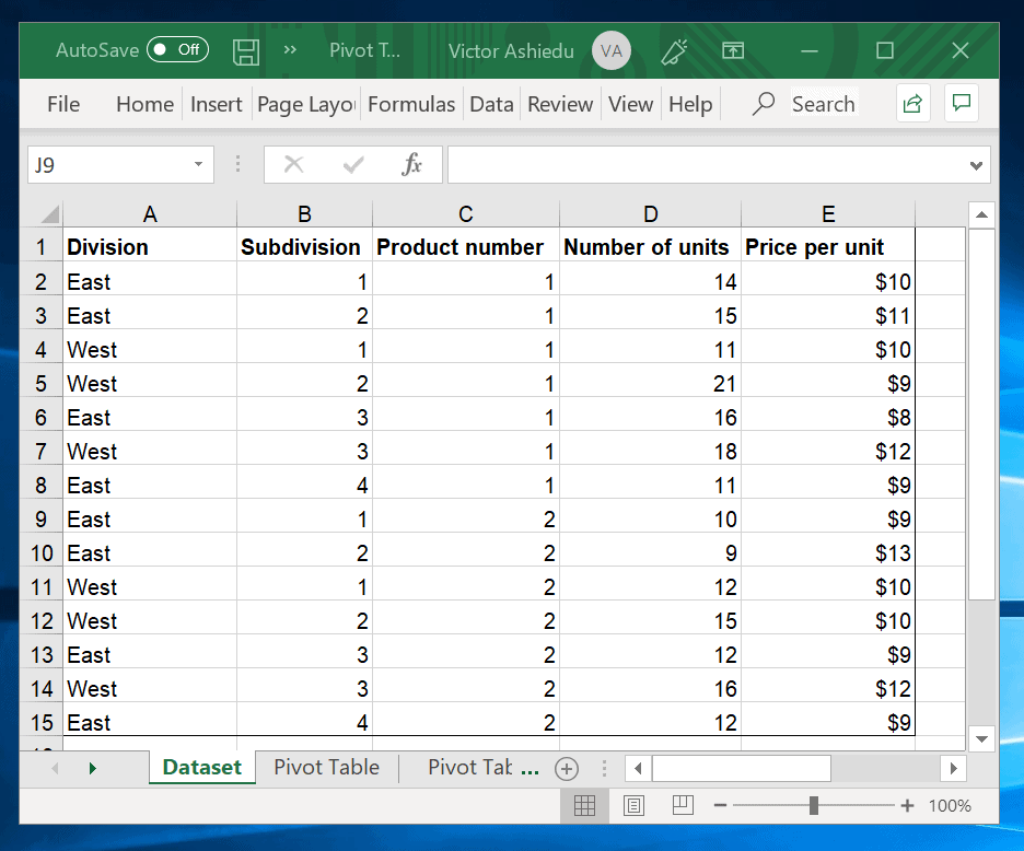
If you are asked to find the average price of products in each division it will be time consuming to get that information directly from the table.
You may also want to know the total number of products in each division, by subdivision. A Pivot Table will help you easily group the data so as to extract and analyze the data.
You can make a Pivot Table using Excel’s recommended PivotTables. You could also make a Pivot Table from a blank PivotTable. In the next two sections, I will demonstrate each.
Option 1: Make a Pivot Table With Excel’s Recommended PivotTables
In this example, I will show you how to make a Pivot Table in Excel using Recommended PivotTables.
Here are the steps:
- Select the data you want to plot a Pivot Table for, including the table headers.
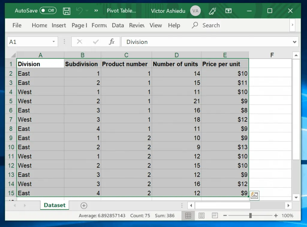
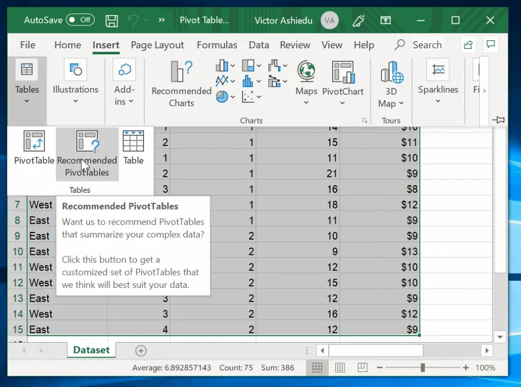
- Click the Insert tab. Then click Recommended PivotTables.
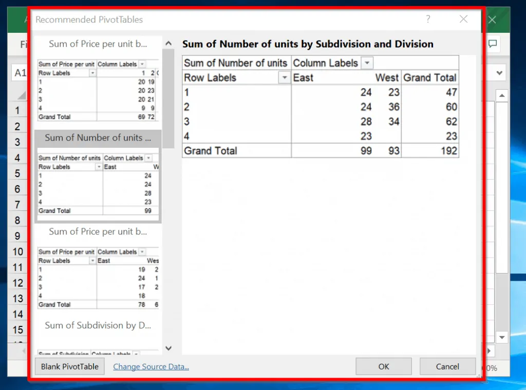
- Excel will open different pre-plotted PivotTables. On the left hand side, select any recommended PivotTable to previou it. Select the one that meets your need. Then click Ok.
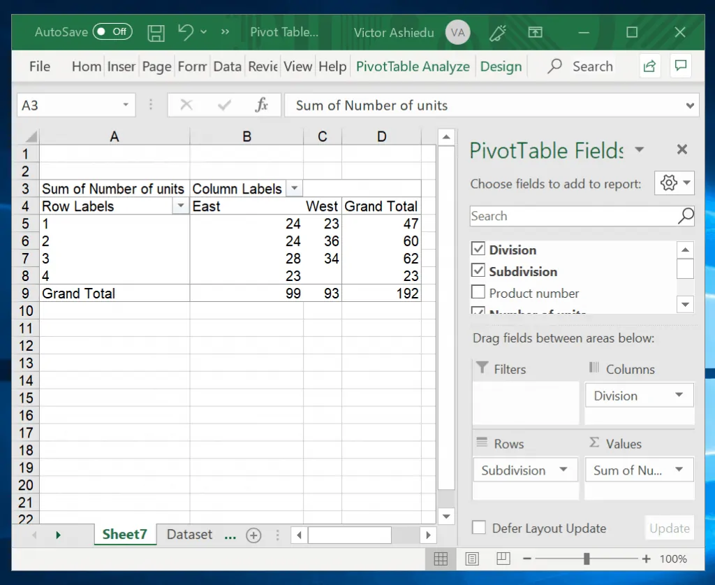
The PivotTable I selected have organized the original data in a way that can be easily analyzed. For the PivotTable to make sense, you will need to change some of the labels. For example, cell A4 is labelled Row Labels. From the original data, this is Subdivisions. Change cell A4 to Subdivision.
Also, cell B3 is called Column Labels. This is Divisions. Change this as well. You may also wish to rename the worksheet to a more recognizable name.
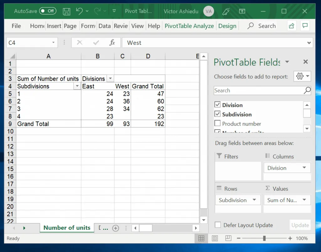
Here is the updated PivotTable.
Option 2: Make a Pivot Table from a Blank PivotTable
You can also make a Pivot Table in Excel from a blank PivotTable.
Here is how:
- Select the data you want to make a Pivot Table from, including the table headers.
- Then click the Insert tab and select PivotTable. The Creat PivotTable option will load.
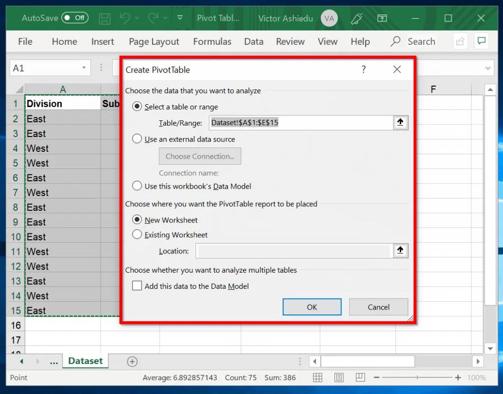
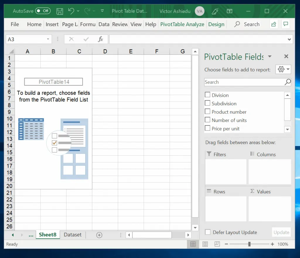
- To create the PivotTable using the default options, click Ok. This will create a blank PivotTable as show below.
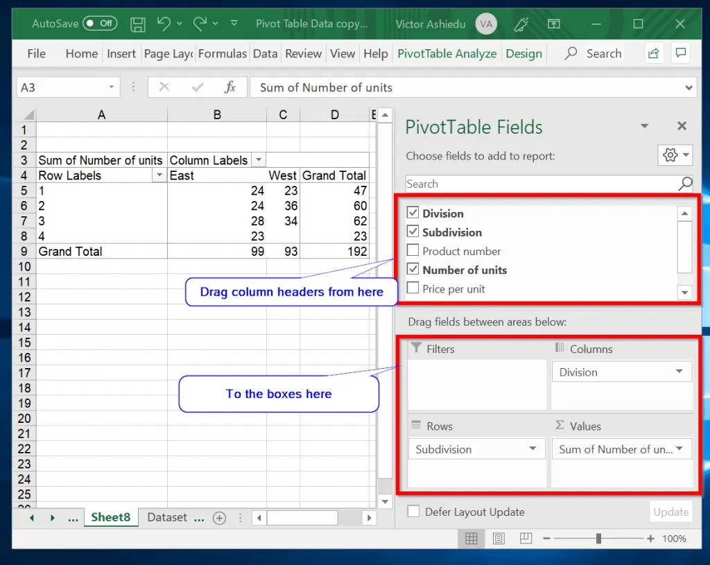
The next step is to insert data into the blank Pivot Table in Excel. This is as simple as dragging and dropping the columns to the Fields, Columns, Rows or Values boxes.
To make a Pivot Table similar to one in the last example:
- Drag Division to Columns box. Then drag Subdivision to Rows box. Finally drag Number of units to Values box. This will produce a Pivot Table as shown in the image below.
How to Customize a Pivot Table in Excel
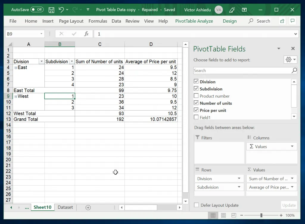
The image below shows a Pivot Table in Excel. It is created from the original data shown in the second image below.
The Pivot Table shows the data organized by Divisions and Subdivisions. It then shows the total units and average Price per unit for each product in a Subdivision.
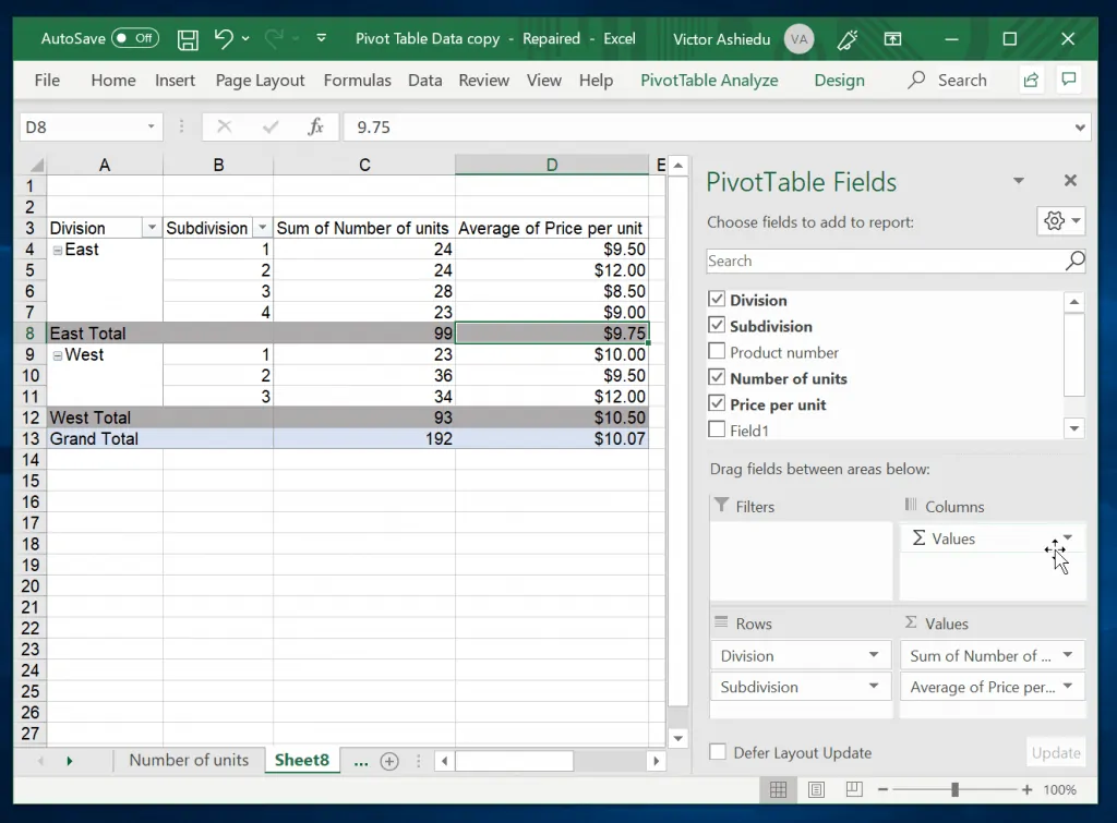
In this section, I will walk you through how to make a Pivot Table similar to the one above.
Here are the steps:
- Create a blank Pivot table using the steps shown in How to Make a Pivot Table in Excel from a Blank PivotTable (link opens in a new browser)
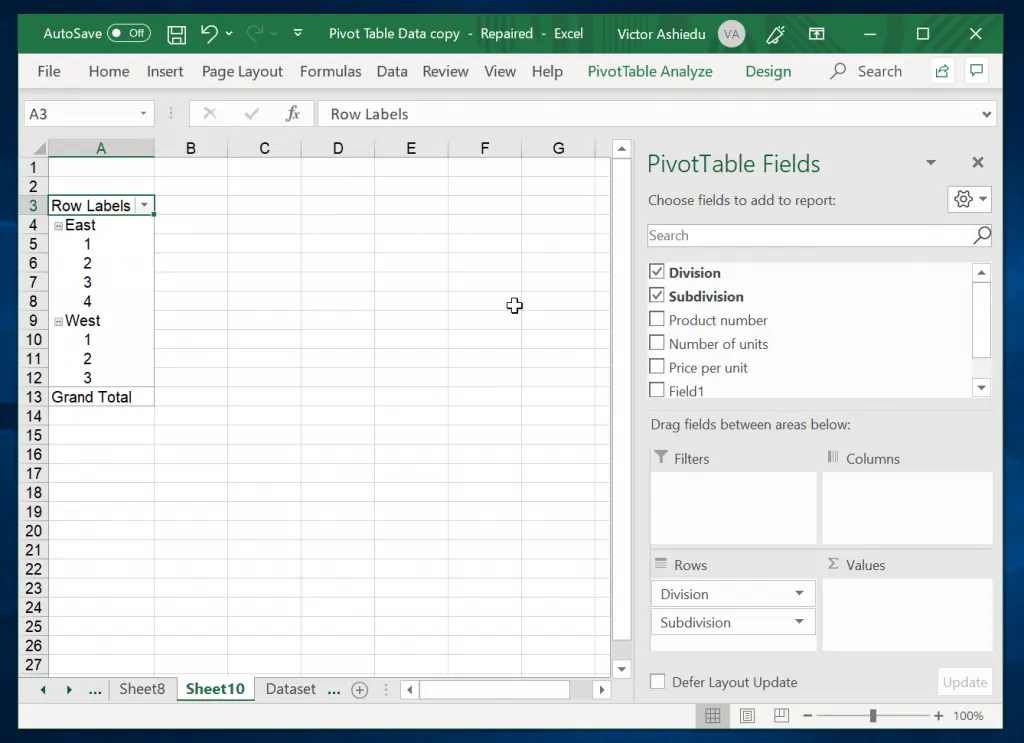
- Next, drag Division and Subdivision columns to the Rows box.
- Then, drag Number of units and Price per unit to the Values box.
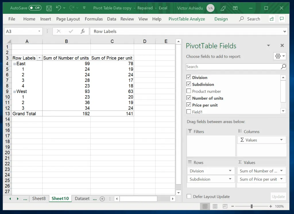
- To turn that column to average, double-click it. It will open for editing.
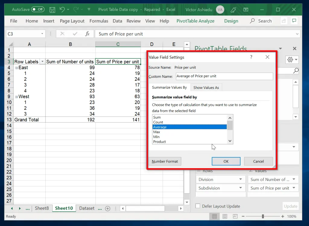
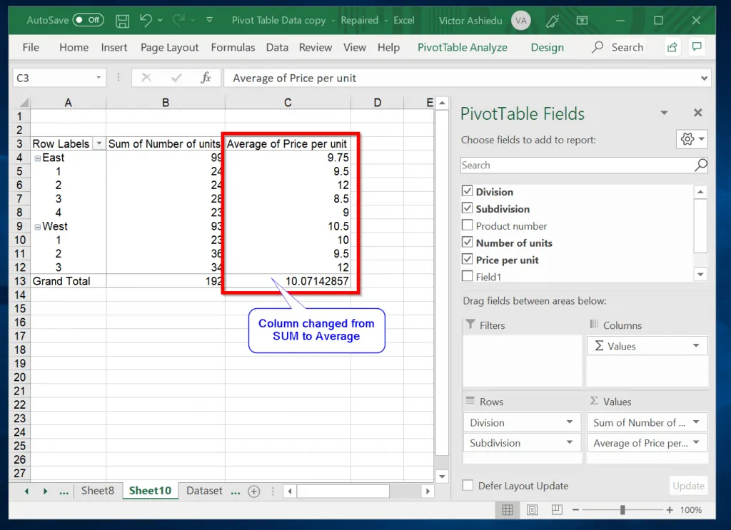
- Beneath the Summarize value field by, select Average. Then click Ok. The column will be changed from Sum to Average. Excel will also label it accordingly.
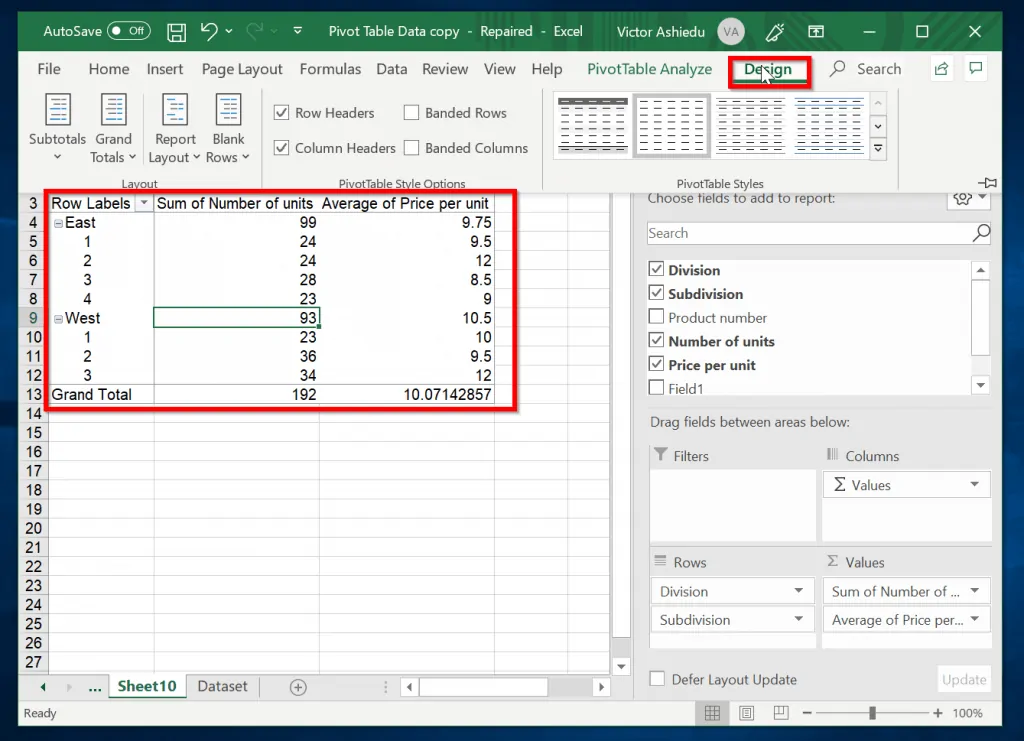
To change the layout to show Division and Subdivision in two separate columns with subtotals:
- Click anywhere on the Table. Then click Design tab.
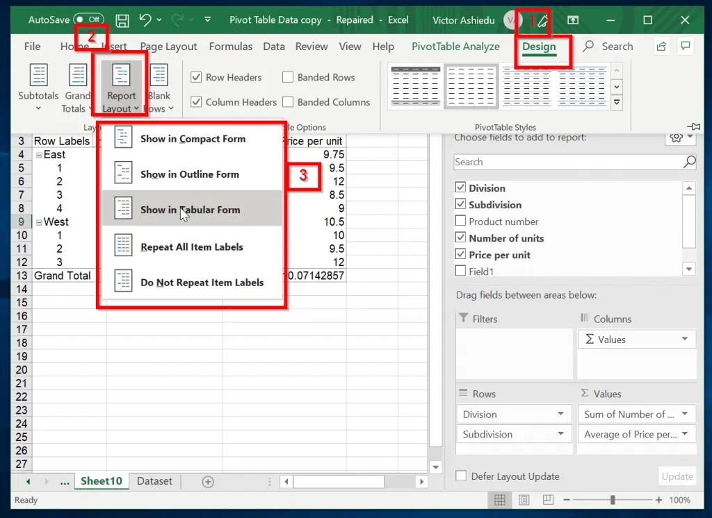
- Next, click the Report Layout drop-down and select a layout. For this guide I will use Show in Tabular Form. The result is shown in the second image below.
Conclusion
This guide showed different ways you can make a Pivot Table in Excel. The guide showed how to make you can make a Pivot Table using Recommended PivotTables.
It also showed how to make one from a blank Pivot Table. Finally, the guide concluded by demonstrating how to customize a Pivot Table in Excel.
If you were able to make a Pivot Table in Excel by following the steps in this guide, kindly spare 2 minutes to share your experience with us. You can respond to the “Was this page helpful?” question below.
Alternatively, share your feedback with our community using the “Leave a Reply” form located at the bottom of this page.