
Free tools Windows power users keep installed
One-click scans. No signup required.
Indexing algorithms in vector databases determine how a system finds similar embeddings without comparing every stored vector. Flat search gives exact results, HNSW usually offers the strongest general-purpose latency–recall balance, IVF reduces search work through clustering, and quantized or disk-based indexes reduce memory requirements. The best choice depends on scale, filters, updates, hardware, and recall targets.
A vector index is not automatically an improvement over a full scan. For a small collection, a highly selective filter, or an evaluation workload, exact search can be faster operationally and provides the ground truth needed to measure approximate recall. At larger scale, approximate nearest-neighbor (ANN) indexes reduce the number of vectors examined, trading some combination of accuracy, memory, build time, update complexity, and tuning effort for speed.
Key takeaways
- Exact or flat search scans the stored vectors and provides perfect recall relative to the collection, making it the baseline for small datasets, selective filters, and evaluation.
- HNSW is a strong starting point for interactive, high-recall search when the graph and vectors fit comfortably in memory, but HNSW generally costs more RAM and build time than IVFFlat.
- IVF searches selected centroid lists using
nprobeorprobes; pgvector documents starting heuristics of approximatelyrows / 1000lists up to one million rows and approximatelysqrt(rows)lists above one million rows. - Scalar quantization, product quantization, binary quantization, and disk-oriented indexes can reduce memory pressure, but their recall and latency must be measured against an exact baseline.
- Metadata filtering can reduce the number of usable ANN candidates, so filtered recall, not just unfiltered recall, must be part of index selection and testing.
- A dedicated vector database is not mandatory: pgvector may be the simplest choice for an existing PostgreSQL application, while FAISS may be sufficient for an embedded or offline similarity-search service.
What is a vector index and why is it needed?
A vector index is an auxiliary data structure that helps a search system find the nearest stored vectors while examining fewer candidates than a brute-force scan. An application first converts a query into an embedding, selects a distance metric, asks the index for candidates, applies filtering, optionally reranks the candidates with more precise distance calculations, and returns the top k results.
Embeddings are points in a high-dimensional space. Similarity is usually measured with Euclidean distance, cosine distance or similarity, or inner product rather than with a simple text or numeric ordering. A conventional B-tree remains useful for scalar metadata such as tenant IDs, timestamps, and categories, but a B-tree does not directly preserve all neighborhood relationships in a high-dimensional embedding space.
#1 Best Overall
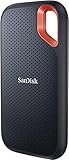
- Get NVMe solid state performance with up to 1050MB/s read and 1000MB/s write speeds in a portable, high-capacity drive(1) (Based on internal testing; performance may be lower depending on host device & other factors. 1MB=1,000,000 bytes.)
- Up to 3-meter drop protection and IP65 water and dust resistance mean this tough drive can take a beating(3) (Previously rated for 2-meter drop protection and IP55 rating. Now qualified for the higher, stated specs.)
- Use the handy carabiner loop to secure it to your belt loop or backpack for extra peace of mind.
- Help keep private content private with the included password protection featuring 256‐bit AES hardware encryption.(3)
- Easily manage files and automatically free up space with the SanDisk Memory Zone app.(5). Non-Operating Temperature -20°C to 85°C
The word “index” can describe several different layers:
- Dense-vector index: the flat, HNSW, IVF, PQ, or other structure used for similarity search.
- Payload or metadata index: conventional structures used to find records satisfying filters.
- Sparse or lexical index: structures supporting keyword or sparse-vector retrieval.
- Storage and segment indexes: structures used to locate data, manage immutable segments, and support compaction.
- Routing structures: partitions, shards, replicas, and tenant-specific collections.
- Compression codes: compact representations used to reduce vector memory or accelerate candidate search.
Qdrant, for example, documents its dense-vector HNSW index separately from payload indexes used for filtering and lookup. A payload index is therefore not a replacement for the dense-vector index; production retrieval commonly uses both layers.
How do exact and approximate nearest-neighbor indexes differ?
Exact nearest-neighbor search computes the distance from the query to every eligible stored vector, sorts or selects the closest vectors, and therefore achieves perfect recall relative to the vectors and metric being searched. Approximate nearest-neighbor search uses a shortcut structure to inspect a smaller candidate set, usually improving latency or throughput at the risk of missing some true nearest neighbors.
| Approach | Candidate coverage | Strength | Main cost | Best starting use |
|---|---|---|---|---|
| Exact or Flat | Every eligible vector | Perfect recall baseline and simple behavior | Work grows linearly with collection size | Small collections, validation, reranking, and highly selective filters |
| HNSW | Graph-selected candidates | Strong recall–latency trade-off | RAM, build time, and graph maintenance | Interactive high-recall search with sufficient memory |
| IVF or IVFFlat | Vectors in selected lists | Partitioned search and generally lower build or memory cost than HNSW | Training and nlist/nprobe tuning |
Large or batch-oriented collections with a trained pipeline |
| Quantized index | Compressed vectors or codes | Lower RAM and storage consumption | Approximation and codebook quality can reduce recall | Memory-constrained scale, usually with reranking |
| Disk-oriented graph | Graph and data accessed from storage | Lower dependence on all-data-in-RAM designs | Hardware-sensitive latency and more implementation complexity | Collections too large or expensive to keep entirely in RAM |
FAISS documents IndexFlatL2 and IndexFlatIP as exhaustive indexes. pgvector likewise performs exact nearest-neighbor search by default when an approximate vector index is not being used. Exact search is not merely a fallback: it is the reference against which ANN recall should be measured.
When is exact or flat search the right choice?
Exact search is often the right choice when the collection is small, the filter removes most records before similarity search, or the query rate is low enough that index construction and maintenance would not pay back their cost. Exact search is also appropriate for generating ground-truth results, testing a new embedding model, validating an ANN configuration, and reranking a manageable candidate pool.
Modern flat search can be substantially optimized with SIMD instructions, multithreading, batching, and GPUs. Those optimizations do not change the linear nature of the search, but they can make a full scan practical for workloads that would be unnecessarily complicated with ANN.
FAISS exposes exact indexes such as:
index = faiss.IndexFlatL2(d)
# or, for inner-product similarity:
index = faiss.IndexFlatIP(d)
In PostgreSQL with pgvector, an exact baseline can be run in a transaction by disabling approximate index scans:
BEGIN;

SET LOCAL enable_indexscan = off;
SET LOCAL enable_bitmapscan = off;

SELECT id
FROM items
ORDER BY embedding <=> '[0.1,0.2,0.3]'
LIMIT 10;

COMMIT;
Compare the exact result set with the ANN result set. For top-k retrieval, a simple recall calculation is the number of approximate results also present in the exact top-k, divided by k. For filtered searches, the exact baseline must apply the same filter.
What’s actually slowing this PC down?
Pick the symptom - the matching free tool is one click away.
How does HNSW work?
HNSW, or Hierarchical Navigable Small World, organizes vectors into a multilayer proximity graph. Most vectors appear in the bottom layer, while progressively fewer vectors appear in upper layers that provide longer-range navigation. Search starts in an upper layer, moves greedily toward promising nodes, descends layer by layer, and explores a candidate set in the target layer.
HNSW does not normally require a separate k-means training phase. The graph is built as vectors are inserted, although the exact behavior for updates, deletions, persistence, segments, and compaction depends on the implementation.
Rank #2

- MEET THE NEXT GEN: Consider this a cheat code; Our Samsung 990 PRO Gen4 SSD helps you reach near max performance with lightning-fast speeds; Whether you’re a hardcore gamer or a tech guru, you’ll get power efficiency built for the final boss
- REACH THE NEXT LEVEL: Gen4 steps up with faster transfer speeds and high-performance bandwidth; With a more than 55% improvement in random performance compared to 980 PRO, it’s here for heavy computing and faster loading
- THE FASTEST SSD FROM THE WORLD'S FLASH MEMORY BRAND: The speed you need for any occasion; With read and write speeds up to 7450/6900 MB/s you’ll reach near max performance of PCIe 4.0 powering through for any use
- PLAY WITHOUT LIMITS: Give yourself some space with storage capacities from 1TB to 4TB; Sync all your saves and reign supreme in gaming, video editing, data analysis and more
- IT’S A POWER MOVE: Save the power for your performance; Get power efficiency all while experiencing up to 50% improved performance per watt over the 980 PRO; It makes every move more effective with less consumption
| Parameter | What it controls | Increasing it usually does | Trade-off |
|---|---|---|---|
M |
Target graph connectivity | Improves connectivity and can improve recall | More graph memory and build cost |
efConstruction |
Search breadth while building the graph | Can produce a higher-quality graph | Longer index construction |
efSearch |
Search breadth at query time | Usually improves recall | Higher query latency and working memory |
k |
Requested number of neighbors | Returns a larger result set | May require a larger candidate pool and more reranking |
FAISS describes HNSW’s connectivity parameter M as a major memory and accuracy control. pgvector documents HNSW as having a stronger speed–recall trade-off than IVFFlat in many situations, at the cost of more memory and slower builds.
Why choose HNSW?
- HNSW is a strong general-purpose choice for low-latency interactive retrieval.
- HNSW can reach high recall by increasing query exploration rather than rebuilding the entire index.
- HNSW commonly supports insertion without a separate global training step.
What can go wrong with HNSW?
HNSW can consume much more memory than the raw vectors alone because the deployment must also hold graph links, IDs, metadata, replicas, segment overhead, query working memory, and the database or application process. High-ingest workloads can also make graph maintenance, deletion handling, and compaction expensive.
Do these 3 things before closing this tab:
1Clear out junk files and repair common Windows errors2Fix the driver behind crashes, sound loss and screen glitches3Repair Windows errors before they cause bigger problemsFiltering is another failure mode. If the graph search examines too few nodes and a post-search filter removes most of those nodes, the query can return fewer than k results even though enough matching records exist. Increasing efSearch, using iterative filtering where supported, or switching to a filter-aware execution strategy can help.
A practical HNSW tuning sequence is to establish exact recall, choose a reasonable graph configuration, increase efSearch until recall reaches the target, and then measure p95 and p99 latency at realistic concurrency. Do not select the highest-recall setting solely from a single warm-cache query.
How does IVF or IVFFlat work?
IVF, or an inverted file index, divides the vector space into coarse regions called lists. A training stage usually learns centroids with a clustering method such as k-means. During a query, the system finds the nearest centroids and searches only the corresponding lists.
- Train a coarse quantizer using representative vectors.
- Assign database vectors to their nearest centroid or centroids.
- At query time, identify the nearest centroids to the query.
- Search the selected lists.
- Optionally rerank the candidates with full-precision vectors.
The most important controls are nlist or lists, which determines the number of partitions, and nprobe or probes, which determines how many partitions are searched. Too few lists can leave each list very large; too many lists can make training and list management inefficient. Too few probes reduce recall, while too many probes approach exhaustive search and reduce the speed advantage.
For pgvector, the documented starting heuristics are approximately rows / 1000 lists for datasets up to one million rows and approximately sqrt(rows) lists for larger datasets, with approximately sqrt(lists) probes as an initial query-time setting. These are tuning starting points, not guarantees. IVFFlat should generally be created after the table contains representative data because the index needs training.
CREATE INDEX items_embedding_ivfflat
ON items
USING ivfflat (embedding vector_cosine_ops)
WITH (lists = 100);

SET ivfflat.probes = 10;
IVF quality depends on the training sample. A sample that does not represent languages, tenants, categories, time periods, or other subpopulations in production can produce poorly placed vectors and uneven list sizes. If the corpus distribution changes substantially, retraining or rebuilding may be necessary.
IVF often uses less memory and builds faster than an uncompressed HNSW index in documented implementations, but the actual result depends on vector dimensions, IDs, list structure, compression, graph settings, and storage format. Cluster imbalance can also create hotspots and uneven latency.
What do scalar quantization, product quantization, and binary quantization do?
Quantization stores an approximation of a vector using fewer bits. Compression can make a larger working set fit in memory, reduce storage traffic, and speed up distance calculations, but it can alter the nearest-neighbor ordering. Quantization should therefore be evaluated as an accuracy–resource trade-off, not as a universally free optimization.
Recommended Free Tools
Rank #3

- THE SSD ALL-STAR: The latest 870 EVO has indisputable performance, reliability and compatibility built upon Samsung's pioneering technology.Computer Platform:PC.Encryption : Class 0 (AES 256) TCG/Opal v2.0, MS eDrive (IEEE1667), Environmental Specs - Shock : 1,500 G & 0.5 ms (Half sine).
- EXCELLENCE IN PERFORMANCE: Enjoy professional level SSD performance with 870 EVO, which maximizes the SATA interface limit to 560/530 MB/s sequential speeds, Accelerates write speeds and maintains long term high performance with a larger variable buffer
- INDUSTRY DEFINING RELIABILITY: Meet the demands of every task from everyday computing to 8K video processing, with up to 2,400 TBW
- MORE COMPATIBLE THAN EVER: 870 EVO has been compatibility tested for major host systems and applications, including chipsets, motherboards, NAS, and video recording devices. Interface- SATA 6GB/s, compatible with SATA 3GB/s and SATA 1.5GB/s interfaces
| Technique | Basic idea | Typical advantage | Important risk |
|---|---|---|---|
| Scalar quantization (SQ) | Represent each floating-point component with fewer bits | Simple memory reduction and fast approximate distances | Component-level precision loss |
| Product quantization (PQ) | Split vectors into subvectors and encode each with a trained codebook | Substantial compression, often combined with IVF | Codebook quality and code size affect recall |
| Optimized or rotated PQ | Transform the vector before product quantization | Can make dimensions more suitable for compression | Additional training and implementation complexity |
| Binary quantization | Represent vector information in binary codes | Very compact and fast Hamming-style comparisons | Usually requires careful validation and reranking |
FAISS documents PQ, IVF-PQ, scalar quantizers, and refinement indexes. Weaviate also documents product and rotational quantization as ways to reduce HNSW resource consumption.
A common architecture searches compressed codes to produce a broad candidate set, then reranks those candidates using the original or higher-precision vectors. Reranking improves quality but requires retaining the original vectors or accessing them from storage. If the original vectors are discarded, the system cannot recover precision that was lost during compression.
Quantization quality can vary across languages, categories, model subpopulations, and long-tail queries. Test a representative validation set and include filtered queries. A quantizer trained on yesterday’s corpus may degrade after a substantial embedding-model or data-distribution change.
When should you use disk-based, GPU, or hybrid indexes?
Disk-oriented indexes such as DiskANN- or Vamana-style systems matter when the collection is too large or too expensive to keep entirely in RAM. These indexes trade some simplicity and often some latency for lower memory dependence and storage-oriented scaling. A disk-oriented index is not automatically faster or cheaper than HNSW: hardware, cache behavior, filters, concurrency, replication, and implementation determine the result.
PC Slower Than It Used to Be?
A free scan shows the junk files, broken settings and background clutter dragging Windows down - then fixes them in one click.Free scan · Windows 10 & 11Outdated Drivers Are Slowing You Down
One free scan finds every outdated or missing driver and matches the right update for your exact hardware.Free scan · exact hardware matchScaNN combines partitioning, quantization, and candidate-search techniques and is exposed by some systems rather than universally. GPU-oriented indexes, including systems such as CAGRA in supported environments, can be attractive when GPU construction and query capacity are available and economically justified. GPU performance must include transfer costs, batching behavior, utilization, and the cost of keeping data available to the accelerator.
Hybrid designs are common. Examples include IVF-PQ, HNSW over compressed vectors, compressed candidate search followed by exact reranking, or ANN combined with metadata indexes and tenant routing. Milvus documentation lists FLAT, IVF variants, HNSW variants, and SCANN, but exact availability and hardware support must be checked against the target Milvus release and deployment mode.
How does metadata filtering change ANN behavior?
Metadata filtering can change the best index choice because a filter may eliminate most of the candidates generated by an otherwise excellent ANN search. Filtering may occur before traversal, during candidate generation, after ANN candidate generation, through an iterative scan, or through partitioning and filter-aware structures. The execution strategy is an implementation property, not something that can be inferred from the algorithm name alone.
| Filter pattern | Likely problem | Useful starting response |
|---|---|---|
| Matches about 1% of the collection | Most ANN candidates are discarded | Use filter-aware or iterative search, increase exploration, add metadata indexes, or consider exact search over the eligible subset |
| Matches about 50% of the collection | ANN usually has a larger eligible pool, but candidate depth can still matter | Benchmark normal ANN settings and compare filtered recall |
| One tenant among many | Global graph traversal may waste work or return too few tenant-qualified candidates | Use tenant partitioning, isolated collections, or filter-aware search where justified |
| Time range | Recent records may be a small or uneven portion of the corpus | Combine scalar indexes, time partitions, and a sufficiently broad ANN candidate search |
| Several predicates | Predicate selectivity and execution order become important | Inspect the query plan and test the complete predicate combination |
| No eligible record exists | Returning fewer than k results is correct |
Define and test an explicit empty-result behavior |
Fewer than k eligible records exist |
The query cannot return k valid results |
Return the available records rather than treating the result as an ANN failure |
pgvector warns that approximate indexes can return fewer results when filtering is applied after the index scan. Its iterative scans can continue expanding the scan until enough filtered results are found or a configured limit is reached, with strict and relaxed ordering modes.
Quick wins for a faster PC:
Fix the driver behind crashes, sound loss and screen glitchesFind Drivers →Repair Windows errors before they cause bigger problemsFix Now →SET hnsw.iterative_scan = strict_order;
SET hnsw.max_scan_tuples = 20000;
SET hnsw.scan_mem_multiplier = 2;For an IVFFlat index, pgvector documents corresponding iterative-scan controls such as:
SET ivfflat.iterative_scan = relaxed_order;
SET ivfflat.max_probes = 100;
Strict ordering prioritizes exact result order, while relaxed ordering can search more broadly and may return results that are slightly out of order until a final sort or reranking step. Check the installed pgvector release because defaults and available controls can change.
Rank #4
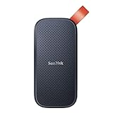
- Solid state performance with up to 800MB/s read speeds in a portable drive. (Based on internal testing; performance may be lower depending on host device, interface, usage conditions and other factors. 1MB=1,000,000 bytes.)
- Back up your content and memories on a storage solution that fits seamlessly into your mobile lifestyle.
- Take it with you on your adventures—up to two-meter drop protection means this durable drive can take a beating. (Based on internal testing.)
- Secure it to your belt loop or backpack for extra peace of mind thanks to the tough rubber hook.
- From Sandisk, a brand professional photographers trust to take on assignments.
Other remedies include conventional indexes on tenant IDs and timestamps, partial indexes for a small number of fixed categories, explicit partitions, separate tables or collections for strong tenant isolation, and exact search over a highly selective candidate set. Partitioning can improve routing but too many small partitions create operational overhead and may waste resources.
How should updates, deletes, and ingestion affect the choice?
Append-heavy ingestion is easier than frequent mutation of embeddings, deletes, and metadata. A static benchmark that loads data once and measures queries does not represent a production system with continual ingestion.
- Append-heavy data: IVF can work well when periodic training and batch building are acceptable; HNSW can accept inserts in common implementations.
- Frequently updated embeddings: Confirm whether the engine updates graph entries in place, writes new segments, or relies on background compaction.
- Deletes: Measure tombstone accumulation, search visibility, compaction, and rebuild behavior.
- Changing distributions: IVF centroids and quantization codebooks may become stale as the corpus or embedding model changes.
- High write concurrency: Measure the effect of ingestion on query latency, memory, locks, background work, and replica lag.
- Recovery: Record how long a full index rebuild takes and whether search remains available during rebuilding.
Index selection should include update latency, delete visibility, compaction time, rebuild time, and ingestion throughput—not just a static query latency number.
How do major vector systems expose indexing algorithms?
Product names and algorithm names are not interchangeable. A vendor may expose a public index family, hide implementation details behind an adaptive service, or combine several structures internally.
| System | What current documentation describes | What to verify in a deployment |
|---|---|---|
| pgvector | Exact search by default, HNSW, IVFFlat, iterative scans, and several vector types | Extension version, memory, filtering plan, PostgreSQL scaling, vacuum, and replication behavior |
| FAISS | A broad similarity-search library including Flat, HNSW, IVF, SQ, PQ, binary, and composite indexes | Persistence, filtering, service layer, concurrency, monitoring, and distributed behavior that your application must provide |
| Weaviate | HNSW, Flat, Dynamic, and HFresh in current documentation; HNSW is generally recommended and Flat suits low object counts per index | Target Weaviate version, experimental status of Dynamic, compression settings, multi-tenancy, and managed-service limits |
| Qdrant | HNSW for current dense-vector indexing plus separate payload indexes | Filter execution, segment behavior, replicas, collection design, and cloud or self-hosted operational limits |
| Milvus | FLAT, IVF variants, HNSW variants, and SCANN among its documented families | Release, vector type, hardware support, distributed deployment, and index-specific resource requirements |
| Pinecone | Managed adaptive selection: its documentation describes Ananas for small slabs, PQFS for medium slabs, and IVF with PQFS for large slabs | Current service behavior, plan limits, filter performance, exportability, and total cost |
Pinecone describes adaptive proprietary algorithm selection by data-slab size rather than requiring every customer to select a public HNSW or IVF configuration. This is useful operationally for teams that prefer a managed service, but it reduces direct control and makes black-box workload testing especially important.
Weaviate’s current documentation lists HNSW, Flat, Dynamic, and HFresh; the documentation describes Dynamic as experimental and available beginning in Weaviate version 1.25. Qdrant’s current documentation describes HNSW for dense vectors, but Qdrant’s payload indexes and other search features remain separate. Both statements should be checked against the release and deployment being evaluated.
The Tool Desk
Outbyte PC Repair FREERepair Windows errors before they cause bigger problemsFix Now →Outbyte Driver Updater FREEFix the driver behind crashes, sound loss and screen glitchesFind Drivers →How do you choose between pgvector, FAISS, and a dedicated vector database?
Choose the system boundary before choosing the ANN algorithm. The right question is not only “Which index is fastest?” but also “Which system can provide the required filtering, transactions, availability, isolation, scaling, backups, and operational workload?”
| Situation | Strong starting option | Why | Main caution |
|---|---|---|---|
| Existing PostgreSQL application with moderate vector workloads | pgvector | Joins, transactions, scalar indexes, backups, and vector search in one operational system | Memory, vacuum, partitioning, and horizontal scaling still require planning |
| Embedded application or offline batch similarity search | FAISS | Broad algorithmic toolkit without a server dependency | You must build persistence, filtering, access control, monitoring, and lifecycle management |
| Managed vector service with minimal database operations | Pinecone, Qdrant Cloud, or Weaviate Cloud | Managed scaling, availability, and service integrations | Pricing, vendor-specific limits, lock-in, and algorithm opacity |
| Large configurable distributed deployment | Milvus or a comparable dedicated system | Multiple index families and distributed operation | More operational complexity and release-specific tuning |
A dedicated vector database becomes more compelling when vector search needs independent scaling, high concurrency, distributed availability, specialized filtering, or large-scale ingestion. pgvector is often simpler when relational data and vector data must remain transactionally connected. FAISS is often enough when the application needs a library and the surrounding service can supply the missing database capabilities.
Independent reader supportYour contribution helps us test, update, and keep practical guides available for everyone.What is a practical tuning methodology?
- Define the metric. Confirm whether the model and application require L2 distance, cosine distance, inner product, or Hamming distance for binary vectors. Confirm whether vectors are normalized. With normalized vectors, cosine similarity and inner product are closely related, but the operator and sort direction still need to be correct.
- Create exact ground truth. Run exhaustive search on representative queries, including every important metadata-filter pattern.
- Set a task target. Choose the required recall@
k, acceptable p95 and p99 latency, throughput, freshness, and resource budget. - Choose a simple baseline. Start with Flat for small collections, HNSW for a memory-rich interactive workload, or IVF when a trained partitioned pipeline is appropriate.
- Tune one variable at a time. For HNSW, vary
efSearchbefore changing graph construction. For IVF, vary probes and then reassess list count. For compression, compare code sizes and reranking depth. - Measure concurrency. Record p50, p95, and p99 latency at the concurrency the application will actually use. Include warm and cold cache conditions where relevant.
- Measure resources. Record RAM per vector, storage per vector, CPU or GPU utilization, build time, ingestion throughput, and rebuild time.
- Test mutations. Add updates, deletes, compaction, and search-visibility checks to the benchmark.
- Test filters. Include 1%-selectivity, 50%-selectivity, single-tenant, time-range, multi-predicate, empty, and underfilled-result cases.
- Test the application. In RAG, retrieval recall is not the same as answer quality. Evaluate chunking, reranking, context limits, duplicate results, freshness, and answer faithfulness as well.
Do not compare a local FAISS process with a distributed managed database as though they share the same system boundary. Account separately for network latency, shard fan-out, global top-k merging, replicas, storage, backups, and managed-service overhead. Also avoid comparing different embedding models, dimensions, metrics, k values, cache states, or index configurations.
A recent 2026 evaluation of multiple vector systems examines performance, quality, and resource trade-offs. Numerical benchmark conclusions still require inspection of the paper’s datasets, hardware, versions, and configurations before being generalized to another deployment.
Best Value

- HUGE SPEED BOOST: Get random read/write speeds that are 40%/55% faster than 980 PRO; Experience up to 1400K/1550K IOPS, while sequential read/write speeds up to 7,450/6,900 MB/s reach near the max performance of PCIe 4.0*
- BREAKTHROUGH POWER EFFICIENCY: Use less power and get more performance; Enjoy up to 50% improved performance per watt over 980 PRO, plus optimal power efficiency with max PCIe 4.0 performance**
- SMART THERMAL CONTROL: Samsung's own nickel-coated controller delivers effective thermal control; With its slim size, 990 PRO is a perfect fit for desktops and laptops that meet the PCI-SIG D8 standard***
- THE CHAMPION MAKER: Up to 65% improvement in random performance enables faster loads for an ultimate gaming experience on PS5 and DirectStorage PC games****
- SAMSUNG MAGICIAN SOFTWARE: Get the most out of your SSD with Samsung Magician's advanced yet intuitive optimization tools; Monitor drive health, protect valuable data, and receive important updates for your 990 PRO
How do you diagnose low recall or missing filtered results?
Low recall usually means the search is exploring too little of the index, the index was built or trained poorly, the metric is wrong, compression is too aggressive, or filtering removes candidates before enough valid results are found.
| Symptom | Likely cause | Diagnostic or remedy |
|---|---|---|
| Low unfiltered recall with HNSW | efSearch is too low or graph construction is weak |
Increase efSearch; then test M and efConstruction against build and memory budgets |
| Low unfiltered recall with IVF | Too few probes, poor list count, or unrepresentative training | Increase nprobe; inspect list balance and retrain with representative vectors |
| Recall falls only after compression | Quantization error or insufficient reranking | Use more precise codes, retain original vectors, enlarge the candidate pool, or rerank more candidates |
Fewer than k filtered results |
Post-ANN filtering discarded too many candidates | Use iterative scans, increase exploration, add metadata indexes, partition, or use exact search for selective filters |
| IVFFlat performs poorly immediately after creation | Too little data was available for training relative to list count | Build after representative data is present and reassess list and probe settings |
| Unexpectedly poor similarity ordering | Metric, normalization, operator, or sort direction mismatch | Validate embedding normalization and compare against a trusted exact calculation |
| Recall degrades over time | Data distribution drift, stale codebooks, tombstones, or compaction effects | Monitor corpus changes, deletes, segments, and rebuild or retraining procedures |
| Good shard-level results but poor global results | Insufficient shard fan-out or local top-k truncation |
Increase local candidate depth and verify global merge behavior |
Use PostgreSQL’s EXPLAIN (ANALYZE, BUFFERS) when working with pgvector:
EXPLAIN (ANALYZE, BUFFERS)
SELECT id, metadata
FROM items
WHERE category_id = 123
ORDER BY embedding <=> '[0.1,0.2,0.3]'
LIMIT 10;
Check whether the expected index is used, how many candidates are examined, whether filtering is applied before or after ANN traversal, and whether the actual execution plan changes at different selectivities.
What changes in distributed vector search?
Distributed vector search adds network and coordination costs to local ANN behavior. A query may fan out to several shards or segments, each shard may produce a local top-k, and a coordinator must merge those results into a global top-k.
The Tool Desk
Outbyte Driver Updater FREEScan for outdated or missing drivers - takes under a minuteDriver Scan →Outbyte PC Repair FREERepair Windows errors before they cause bigger problemsFix Now →- Shard fan-out: More shards can increase parallelism but also add network and merge overhead.
- Local candidate depth: Returning too few candidates from each shard can cause the global result to miss a true neighbor.
- Filtering: A tenant or time filter may be local to some shards or require broad fan-out.
- Hot partitions: Uneven tenant or centroid distribution can make one shard the latency bottleneck.
- Replicas: Replica selection affects load balancing, freshness, and tail latency.
- Rebalancing: Moving data can require index transfer, rebuilding, or temporary resource headroom.
A single-node FAISS measurement is therefore not directly comparable with a managed distributed database measurement. State the system boundary, hardware, concurrency, data placement, and network path in every benchmark.
Production checklist
- Confirm the embedding model, vector dimension, normalization, distance metric, and operator.
- Pin and record database, extension, library, server, GPU, and index versions.
- Keep an exact-search recall regression test with representative unfiltered and filtered queries.
- Monitor p50, p95, and p99 latency, QPS, error rate, and result-count shortfalls.
- Monitor raw-vector memory, graph or code memory, metadata memory, replicas, and query working memory.
- Record index-build, training, compaction, ingestion, update, delete, and rebuild times.
- Test highly selective filters, multi-tenant queries, time ranges, empty results, and requests larger than the eligible population.
- Define how deleted and updated records become searchable or disappear from results.
- Document iterative-scan, probe, exploration, reranking, and fallback settings.
- Plan backups, restoration, index rebuilding, rollback, and capacity headroom.
- Measure total cost, including compute, storage, replicas, backups, network egress, and operational labor.
- Rebenchmark after changing the embedding model, corpus distribution, tenant mix, hardware, or software version.
Final decision matrix
| Primary workload condition | Starting point | Why it fits | What to validate first |
|---|---|---|---|
| Small collection or highly selective filter | Exact or Flat | Perfect recall and minimal index complexity | Full-scan latency and eligible-row count |
| Interactive high-recall search with ample RAM | HNSW | Strong recall–latency balance | Memory per vector, filtered recall, and tail latency |
| Batch ingestion with a trained pipeline | IVF or IVFFlat | Searches selected partitions and can build efficiently | Training quality, list balance, probes, and rebuild cadence |
| Memory-constrained large collection | IVF-PQ, scalar-quantized HNSW, or another compressed design | Reduces RAM and storage requirements | Recall loss, reranking depth, and codebook drift |
| Collection too large for an economical all-RAM design | Disk-oriented graph or hybrid index | Reduces RAM dependence | Storage latency, cache behavior, hardware cost, and filtering |
| Existing relational application | PostgreSQL with pgvector | Keeps joins, transactions, filters, and vectors together | Database resource contention, scaling, and maintenance |
| Embedded or offline application | FAISS | Provides a broad set of similarity-search primitives | Persistence, filtering, service APIs, monitoring, and concurrency |
| Managed specialized retrieval platform | Pinecone, Qdrant Cloud, Weaviate Cloud, or Zilliz Cloud | Reduces infrastructure operations | Filtered recall, total cost, scaling limits, exportability, and lock-in |
There is no universally best vector-database indexing algorithm. Flat search is the quality baseline; HNSW is the usual first experiment for memory-rich interactive retrieval; IVF is a strong candidate when partitioning and training are acceptable; quantization and disk-oriented designs address memory-constrained scale. The final choice should be made from measured recall, filtered behavior, tail latency, throughput, lifecycle costs, and operational requirements.
Frequently Asked Questions
What is the best indexing algorithm for a vector database?
There is no universally best vector-database indexing algorithm. HNSW is a strong starting point for high-recall interactive search with sufficient RAM, while Flat, IVF, quantized, and disk-oriented indexes can be better for small collections, trained batch workloads, memory-constrained scale, or data that cannot economically fit in RAM.
Is HNSW better than IVF?
HNSW is often better for high-recall, low-latency interactive search, while IVF can use less memory and build faster in some implementations. HNSW requires graph memory and maintenance; IVF requires representative training and careful tuning of list count and probes.
How do you measure vector-index recall?
Run exact exhaustive search on the same vectors, metric, filters, and query set, then compare the ANN top-k results with the exact top-k results. Measure filtered recall as well as unfiltered recall, and report latency, throughput, memory, and build time alongside recall.
Does a RAG application need a dedicated vector database?
A RAG application does not necessarily need a dedicated vector database. PostgreSQL with pgvector can be sufficient when relational joins, transactions, and operational simplicity matter, while FAISS can be sufficient for an embedded or offline service; a dedicated system becomes more attractive as scale, concurrency, filtering, availability, and distributed operation grow.
The Bottom Line
Bottom line: Choose the index that satisfies the whole workload, not the one with the most impressive algorithm name. Establish exact ground truth, test realistic filters and mutations, tune one parameter at a time, and compare recall, p95/p99 latency, throughput, memory, build time, recovery, and total cost before committing to HNSW, IVF, compression, a disk-oriented design, or a particular vector platform.
Quick Recap
Product prices and availability are accurate as of the date/time indicated and are subject to change. Any price and availability information displayed on Amazon at the time of purchase will apply.
Quick wins for a faster PC:
Scan for outdated or missing drivers - takes under a minuteDriver Scan →Repair Windows errors before they cause bigger problemsFix Now →Fix the driver behind crashes, sound loss and screen glitchesFind Drivers →
