
iTechGuides is reader-supported. When you buy through links on our site, we may earn an affiliate commission. As an Amazon Associate I earn from qualifying purchases. Learn more
This guide demos how to create a pie chart in Excel and Google Sheets. A pie chart is a circular representation of a data set in portions.
In other words, a pie chart shows portions of a whole set of data in a circular form.




Option 1: Create a Pie Chart in Excel
To create a pie chart in Excel you need a set of data. Here is the data I will use for my demo in this guide.
Outdated Drivers Are Slowing You Down
One free scan finds every outdated or missing driver and matches the right update for your exact hardware.Free scan · exact hardware matchPC Slower Than It Used to Be?
A free scan shows the junk files, broken settings and background clutter dragging Windows down - then fixes them in one click.Free scan · Windows 10 & 11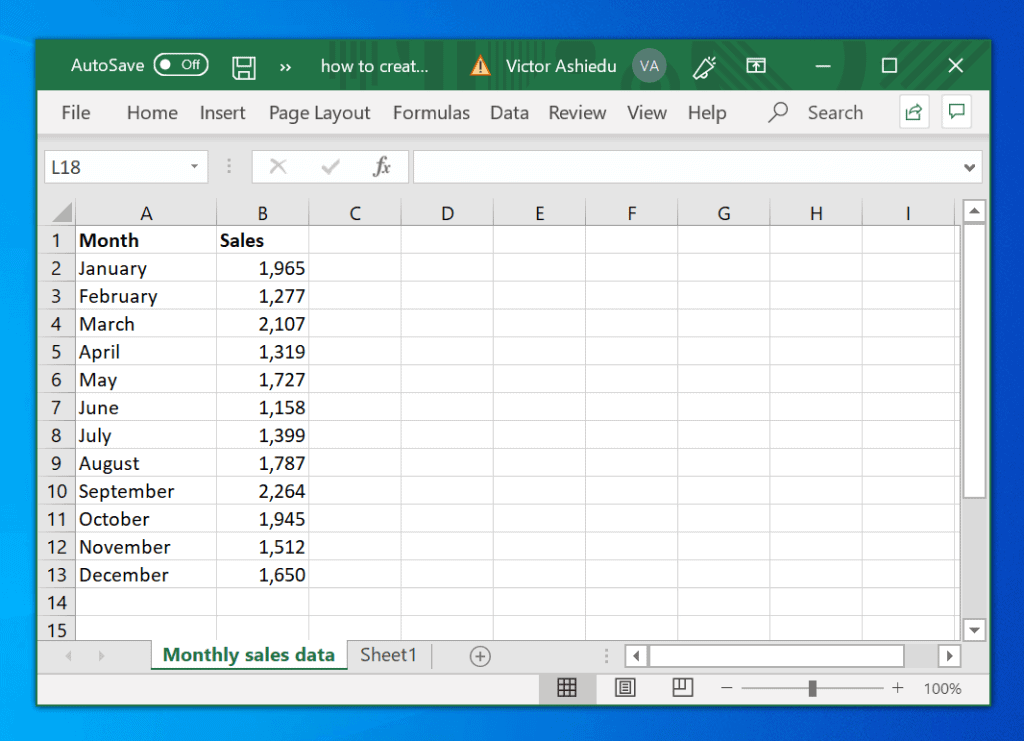
The excel sheet is a monthly sales data for an online retailer.
#1 Best Overall
Here are the steps to create a pie chart in Excel with this data.
- Highlight all the data including its headers.

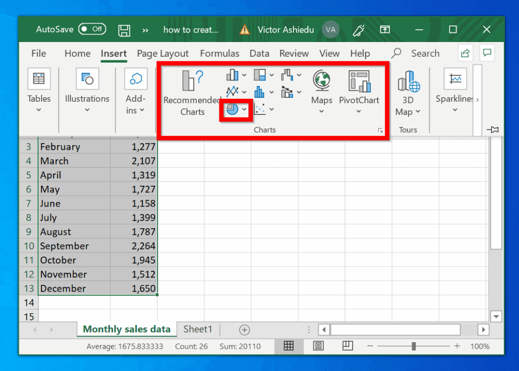
- Then with the data selected, click Insert tab.

- When you click Insert, it will display a set of options. One of them is Charts group (highlighted in the image below).

- In the Charts group, click on Pie chart icon (highlighted in the image below)
- Then select Pie (first option), Pie of pie (second option) or bar of pie (third option). When you hover over a pie chart type, Excel will display the image of the pie chart beneath.


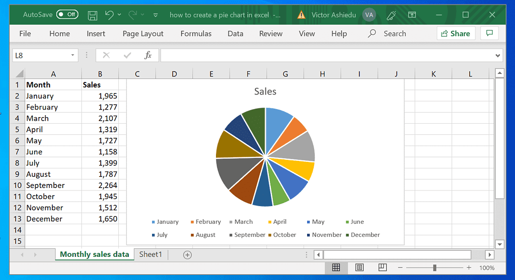
- Once you select a pie chart type, the chart will display on the data. Move the pie chart away from the data.
Option 2: Create a Pie Chart in Google Sheets
Just like excel you can also create a Pie chart in Google Sheets.
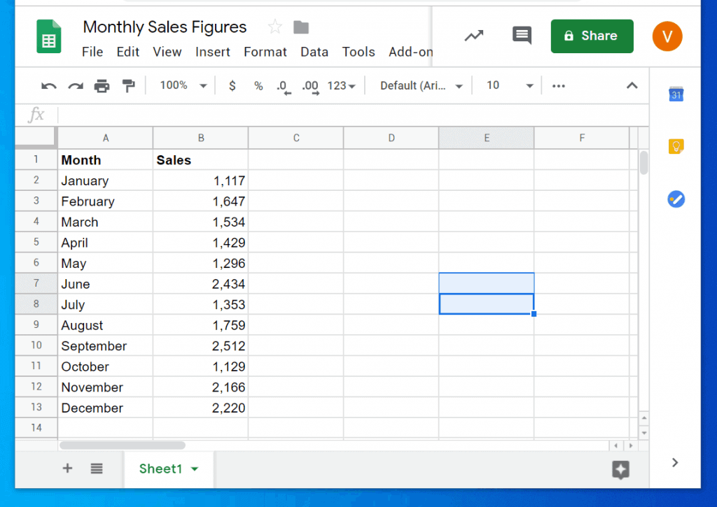
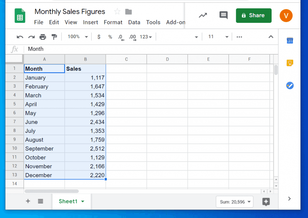
I will use the data in the Google Sheets shown below to demo how to create pie chart in Google Sheets.
Here are the detailed steps to create a pie chart in Google Sheets:
Rank #3

- The Microsoft Office 365 Bible: The Most Updated and Complete Guide to Excel, Word, PowerPoint, Outlook, OneNote, OneDrive, Teams, Access, and Publisher from Beginners to Advanced
- ABIS BOOK
- Highlight all the data including the headers.
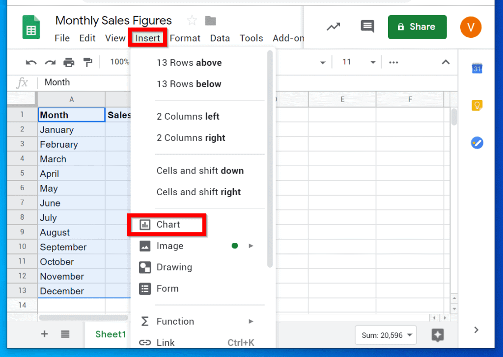
- Then click Insert tab and click Chart.
- When you click Chart, Google Sheets will select Line chart by default. To change the chart type to Pie chart, click the drop-down arrow beside Line chart (see the image below). Then select Pie chart.

- If you wish to customize the chart, click the Customize tab (see the image below).

- Finally, click the x sign on top of the chart insert tool to close it.

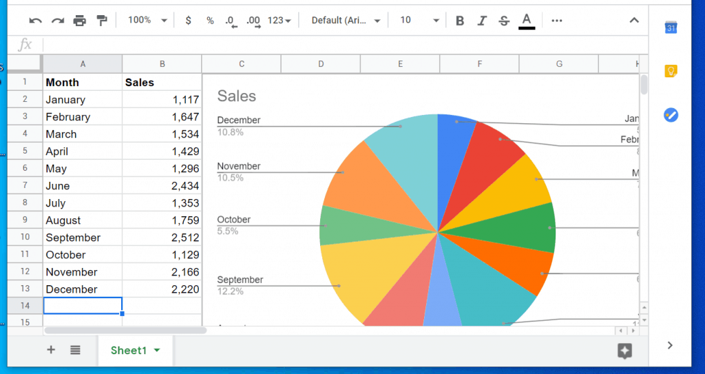
- Then move your pie chart away from your data. You may also resize your chart…
I hope you found this article helpful. If you did, click on “Yes” beside the “Was this page helpful” question below.
You may also express your thoughts and opinions by using the “Leave a Comment” form at the bottom of this page.
For more Windows guides visit our Windows How To page.
Do these 3 things before closing this tab:
1Clear out junk files and repair common Windows errors2Fix the driver behind crashes, sound loss and screen glitches3Repair Windows errors before they cause bigger problemsQuick Recap
Product prices and availability are accurate as of the date/time indicated and are subject to change. Any price and availability information displayed on Amazon at the time of purchase will apply.


