
iTechGuides is reader-supported. When you buy through links on our site, we may earn an affiliate commission. As an Amazon Associate I earn from qualifying purchases. Learn more
There is no single “Indic LLM” hardware requirement. Adapter tuning a 1–3 billion-parameter model can begin with 24–80 GB of VRAM, while full BF16 training needs roughly 12–16 GB of GPU memory per billion parameters before activations and communication buffers. That puts a 2B model around 24–32 GB, an 8B model around 96–128 GB, and a 30B model around 360–480 GB distributed across GPUs.
From-scratch, high-quality pretraining is a cluster project. The decisive variables are training mode, parameter count, context length, batch size, tokenizer efficiency, optimizer, parallelism, interconnect and storage—not the fact that the model supports an Indian language by itself.
Start with the training mode
The same base model can require radically different hardware depending on what you are changing. Quantized adapter training stores only small trainable modules, whereas full pretraining keeps gradients and optimizer state for every parameter. Continued pretraining sits between those extremes but still becomes a full distributed workload as the model grows.
The Tool Desk
Outbyte Driver Updater FREEScan for outdated or missing drivers - takes under a minuteDriver Scan →Outbyte PC Repair FREEClear out junk files and repair common Windows errorsFree Scan →| Training mode | Practical starting point | What it is suitable for |
|---|---|---|
| Adapter or parameter-efficient fine-tuning | 24–80 GB VRAM for a 1–3B base model when quantization and checkpointing are used | Instruction tuning, domain adaptation and experiments on a single workstation or small server |
| Continued pretraining of a 1–3B model | 24–80 GB can be a starting range, depending on sequence length, optimizer and sharding | Adding domain or language data to an existing model |
| Full BF16 training | Approximately 12–16 GB of parameter and optimizer state per billion parameters before activations | Updating every weight in a model |
| From-scratch pretraining at 30B and above | Multi-GPU nodes or a distributed cluster | Building a large general-purpose model with substantial token budgets |
These are planning ranges, not guarantees. Peak allocation rises with sequence length, microbatch size, optimizer implementation, activation storage, communication buffers and framework overhead. A configuration that fits at one context length can run out of memory when the context or batch is increased.
#1 Best Overall

- Data Center Class Reliability: Designed for 24x7 data center operations, ensuring optimum performance, durability, and longevity to meet demanding real-world conditions in machine learning and AI tasks.
- Ampere Architecture: Employs the world's most powerful data center GPU, offering exceptional AI, data analytics, and high-performance computing capabilities.
- Enhanced Tensor Cores: Accelerate deep learning matrix arithmetic at the heart of neural network training and inferencing, resulting in faster and more efficient AI computations.
- High-Speed HBM2e Memory: Equipped with 80GB of high-bandwidth memory, delivering improved raw bandwidth and higher memory bandwidth efficiency for data-intensive AI applications.
- PCIe Gen 4 Support: Provides double the bandwidth of PCIe Gen 3, improving data-transfer speeds for AI and data science workloads, maximizing performance for machine learning tasks.
Convert parameter count into a first-pass VRAM budget
For full mixed-precision Adam-style training, use roughly 12–16 bytes of GPU memory per parameter as an initial estimate. This accounts for weights, gradients and optimizer-related state, but not the activations and temporary buffers that often determine the final peak.
| Model size | Parameter-state estimate before activations | Sensible initial hardware shape |
|---|---|---|
| 1B | 12–16 GB | One 24 GB card for experiments; more capacity for long context or full training |
| 2B | 24–32 GB | One 40–80 GB card or two smaller cards |
| 7–8B | 84–128 GB | At least two 80 GB cards for full training; more for long context |
| 13B | 156–208 GB | Three or more 80 GB cards, depending on sharding and sequence length |
| 30B | 360–480 GB | A multi-GPU node or distributed cluster |
| 70B | 840–1,120 GB | Distributed multi-node training |
For example, the arithmetic for a 2B model is 2 billion parameters multiplied by 12–16 bytes, producing 24–32 GB before activations. The estimate is deliberately conservative about the rest of the system: tensor and pipeline parallelism, data-parallel replicas, communication workspaces and checkpoint staging all consume additional memory.
Why quantization changes the answer
Quantizing the frozen base model can make adapter tuning practical on a much smaller card because the base weights occupy less memory and only the adapter parameters receive gradients. Quantization does not make full-parameter BF16 pretraining fit automatically: gradients, optimizer state and activation memory still have to be allocated for the trainable weights. Treat a quantized single-GPU result as a fine-tuning result, not proof that the same card can pretrain the model.
Quick wins for a faster PC:
Clear out junk files and repair common Windows errorsFree Scan →Scan for outdated or missing drivers - takes under a minuteDriver Scan →VRAM capacity is not the same as compute
VRAM answers “can this step fit?” Compute answers “how quickly can the step run?” Two systems with enough aggregate memory can have very different training times because of accelerator throughput, clock limits, interconnect bandwidth, data-loader performance and scaling efficiency.
Rank #2

- Discrete graphics card memory 40 GB
- Memory bandwidth (max) 1555 GB/s
- Graphics processor family NVIDIA
- Graphics processor A100
Training cost is driven by the number of tokens processed, model size and the work required for each token. Chinchilla’s study of more than 400 models found that compute-optimal training scales model size and training-token count in roughly equal proportion. For an Indic project, apply that principle only after filtering for language balance, script quality, deduplication and contamination. A large but repetitive corpus can waste the same compute that a smaller, cleaner corpus would use more effectively.
Published GPU-hour figures illustrate scale but are not interchangeable benchmarks. Meta reports 3.3 million cumulative GPU hours for Llama 2 pretraining on A100-80GB hardware rated at 350–400 W TDP. Its Llama 3.2 model card lists 370,000 H100 GPU hours for the 1B model and 460,000 H100 GPU hours for the 3B model. Those totals reflect different datasets, software stacks, sequence lengths and training goals, so they should inform order-of-magnitude planning rather than a direct quote for your run.
Indic tokenization can multiply the workload
Token count is especially important for Indian-language training because a tokenizer that represents text inefficiently creates more sequence positions for the same raw corpus. More tokens mean more embedding lookups, attention work, memory traffic, optimizer updates and wall-clock time.
Free tools Windows power users keep installed
One-click scans. No signup required.
Sarvam reports tokenizer fertility of 1.4–2.1 across its supported Indic languages, compared with 4–8 tokens per word for many existing multilingual tokenizers and about 1.4 for English. Fertility varies by language, script and tokenizer, so measure it on your own corpus instead of assuming that a Hindi result applies to every Indic language.
Rank #3
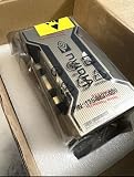
- PERFORMANCE: Features 6,912 CUDA cores and 432 third-gen Tensor cores delivering up to 19.5 TFLOPS FP32 performance for demanding AI and compute workloads
- MEMORY SPECIFICATIONS: Equipped with 80GB of HBM2e memory on a 5120-bit bus, providing massive 2,039 GB/s bandwidth
- ARCHITECTURE: Built on NVIDIA Ampere GA100 architecture with 40MB L2 cache and clock speeds of 1,275 MHz base to 1,410 MHz boost
- CONNECTIVITY: Features NVLink technology with 600 GB/s bandwidth for high-speed multi-GPU communication
- FORM FACTOR: SXM4 module design with 400W TDP, supporting up to 7 MIG partitions for workload optimization
What to benchmark before buying GPUs
- Tokens per word for each target language and script.
- The share of text that falls back to byte or character-level pieces.
- Average and worst-case sequence length after packing.
- Padding waste at your planned batch and context sizes.
- Token throughput per GPU with the actual model, precision and data pipeline.
Budget in tokens, not documents or words. If a tokenizer produces twice as many tokens for one language, the same document count can require substantially more training steps and storage.
Practical hardware tiers
| Tier | Hardware shape | Use case and limits |
|---|---|---|
| Prototype and data pipeline | One 24–48 GB GPU | Validate tokenization, packing, data loaders, checkpointing and small adapter runs. Use quantization or parameter-efficient methods when the base model does not fit. |
| Small full-model experiments | One 40–80 GB accelerator | Provides room for a 1–3B model, longer sequences and fewer memory compromises. It is a development reference point, not evidence that production pretraining will finish quickly. |
| 7–13B full training | At least two to four 80 GB cards, with sharded optimizer states | Requires fast interconnects. Longer context and larger global batches can push the count higher. |
| 30B and larger | Multi-GPU node or distributed multi-node cluster | Interconnect bandwidth, checkpoint storage, fault recovery and parallelism become first-order constraints. |
Can you train an Indic model on one A100?
An 80 GB A100 is useful for tokenizer development, data-pipeline validation, adapter tuning and some small-model full-training experiments. A 1–3B model can fit in that class of memory with careful precision, sequence and batch settings. Whether it finishes in a reasonable time is a separate question: a single accelerator has limited token throughput and cannot provide the redundancy or aggregate memory of a cluster.
For a 7–8B full-training run, the planning estimate already reaches 84–128 GB before activations, so one 80 GB card is not a comfortable target. Sharding across at least two 80 GB cards is the more realistic starting shape, with additional capacity for long context, larger batches and communication buffers. A 30B run is outside the practical scope of one A100 because its parameter-state estimate alone is 360–480 GB.
What’s actually slowing this PC down?
Pick the symptom - the matching free tool is one click away.
Published Indic training reference points
| Project or report | Published scale | What it demonstrates |
|---|---|---|
| Sarvam-1 | 2B parameters, 10 Indian languages, a corpus described as 2 trillion high-quality Indic tokens | Sarvam says training used 1,024 GPUs for five days on Yotta’s Shakti cluster with NVIDIA NeMo. |
| Sarvam 30B and 105B | Both trained from scratch in India under the IndiaAI mission | Shows the jump from small-model experimentation to national-scale distributed pretraining. |
| Meta Llama 2 | 3.3 million cumulative GPU hours on A100-80GB hardware, listed at 350–400 W TDP | Illustrates the compute budget of a large general-purpose pretraining effort. |
| Meta Llama 3.2 | 370,000 H100 GPU hours for 1B pretraining; 460,000 H100 GPU hours for 3B pretraining | Shows that model size, data and training configuration jointly determine compute. |
| NVIDIA report on Sarvam training | More than 4,096 H100 GPUs | Near-linear scaling was reported with Quantum InfiniBand and Megatron-LM 6D parallelism. |
Sarvam-1’s 1,024-GPU, five-day run is not a minimum requirement for every Indic model. It is a reference point for a 2B model trained on a very large corpus with a production-scale objective. A smaller research run with fewer tokens, shorter context or adapter training is solving a different problem.
Rank #4

- NVIDIA Ampere Architecture-based CUDA Cores - Double-speed processing for single-precision floating point (FP32) operations and improved power efficiency provide significant performance improvements for graphics and simulation workflows, such as complex 3D computer-aided design (CAD) and computer-aided engineering (CAE), on the desktop.
- Second-Generation RT Cores - With up to 2X the throughput over the previous generation and the ability to concurrently run ray tracing with either shading or denoising capabilities, second-generation RT Cores deliver massive speedups for workloads like photorealistic rendering of movie content, architectural design evaluations, and virtual prototyping of product designs. This technology also speeds up the rendering of ray-traced motion blur for faster results with greater visual accuracy.
- Third-Generation Tensor Cores - New Tensor Float 32 (TF32) precision provides up to 5X the training throughput over the previous generation to accelerate AI and data science model training without requiring any code changes. Hardware support for structural sparsity doubles the throughput for inferencing. Tensor Cores also bring AI to graphics with capabilities like DLSS, AI denoising, and enhanced editing for select applications.
- Third-Generation NVIDIA NVLink - Increased GPU-to-GPU interconnect bandwidth provides a single scalable memory to accelerate graphics and compute workloads and tackle larger datasets.
- 48 Gigabytes (GB) of GPU Memory - Ultra-fast GDDR6 memory, scalable up to 96 GB with NVLink, gives data scientists, engineers, and creative professionals the large memory necessary to work with massive datasets and workloads like data science and simulation.
Design the system around parallelism and data movement
Choose the parallelism mix
Data parallelism replicates model work across workers and divides batches. Tensor parallelism splits layer operations across GPUs. Pipeline parallelism divides layers into stages, while expert parallelism is used for mixture-of-experts architectures. The right combination depends on model shape, active parameters, sequence length and the number of GPUs.
For dense models, total parameters determine storage and optimizer-state requirements. For a mixture-of-experts model, active parameters determine per-token compute, while total parameters still affect checkpoint size, routing and memory placement. Do not size an MoE cluster from active parameters alone.
Interconnect determines whether added GPUs help
When workers exchange activations, gradients or expert outputs, link speed and latency can dominate. NVLink inside a node and InfiniBand between nodes are common building blocks for large jobs. NVIDIA reports near-linear scaling above 4,096 H100 GPUs for Sarvam training when InfiniBand and Megatron-LM 6D parallelism were used; that result highlights the software and network conditions required, not a universal scaling guarantee.
PC Slower Than It Used to Be?
A free scan shows the junk files, broken settings and background clutter dragging Windows down - then fixes them in one click.Free scan · Windows 10 & 11Crashes, No Sound, or Screen Glitches?
Random freezes, missing sound and display glitches usually trace back to one bad driver. Find and replace yours safely.Free scan · under a minuteKeep storage ahead of the GPUs
Training data must be read fast enough to keep accelerators busy, and checkpoints must be written without making recovery impractically slow. Use high-throughput local or parallel storage, shard datasets for concurrent readers, and test restart time before a long run. Checkpoint retention also needs a policy: keep enough recent and milestone checkpoints to recover from failures without consuming the entire storage system.
Best Value

- 24GB Video Memory
- Fourth Generation Tensor Cores
- HALF HEIGHT BRACKET ONLY
A repeatable sizing workflow
- Define the objective. Decide whether you are adapter tuning, continuing pretraining or starting from random weights. Record the target languages, scripts, context length and expected number of tokens.
- Measure tokenizer fertility. Tokenize representative samples for every language and calculate tokens per word, fallback rates and packed-sequence length.
- Select parameter count and precision. Use the 12–16 GB-per-billion planning rule for full mixed-precision training, then specify BF16, FP16, FP8 or quantized storage separately.
- Add activation headroom. Test the real sequence length, microbatch and gradient-accumulation settings. Enable activation checkpointing when recomputation is cheaper than storing every activation.
- Choose sharding and parallelism. Decide how optimizer states, gradients, layers and batches will be distributed, then map that plan to the available GPU count and interconnect.
- Estimate throughput in tokens per second. Run a short benchmark with the production model, tokenizer, data format and precision. Convert that rate into tokens per day and expected training duration.
- Plan storage and recovery. Include dataset shards, tokenizer files, optimizer checkpoints, model checkpoints, logs and at least one failure-and-restart test.
- Scale only after profiling. Add GPUs when the current run is compute-bound and communication, input loading and synchronization are not already limiting factors.
Common failure modes and fixes
Out-of-memory errors at the first step
- Lower microbatch size and use gradient accumulation to preserve the global batch.
- Shorten the context temporarily to isolate activation pressure.
- Enable activation checkpointing and use a sharded optimizer.
- Check that the model, gradients and optimizer are using the intended precision.
- Reserve memory for communication workspaces instead of allocating every byte to parameters.
GPUs are allocated but mostly idle
Profile data loading, CPU tokenization, storage reads and inter-GPU synchronization. A fast accelerator cannot compensate for a dataset pipeline that delivers batches late. Pre-tokenizing, increasing parallel readers and placing hot shards on faster storage can remove input stalls.
Scaling becomes slower after adding workers
Measure communication time and per-rank batch size. Excessive tensor or pipeline parallelism can create synchronization overhead, while a slow interconnect can erase the benefit of additional GPUs. Revisit the parallelism split and keep work within a node when the model allows it.
Checkpoints interrupt training for too long
Write checkpoints asynchronously when the framework supports it, keep checkpoint formats consistent, and test restoration on the same number of workers you expect to use in production. A checkpoint that cannot be restored reliably is not a recovery plan.
Loss improves but one language lags
Inspect language proportions, script normalization, duplicate removal and tokenizer fertility by language. A blended loss can hide under-represented languages, so track per-language validation sets and adjust sampling before increasing model size.
What a realistic decision looks like
For a Hindi or multilingual Indic adapter project, a 24 GB GPU can be enough when the base model is quantized, context is moderate and only adapter parameters are trained. For full training of a 1–3B model, move toward 40–80 GB and benchmark the exact sequence and batch settings. For 7–13B models, plan a multi-GPU system with sharded states and a high-speed interconnect. At 30B and above, budget for distributed orchestration, parallel storage, checkpoint recovery and network engineering rather than treating the job as a larger single-GPU experiment.
The most defensible estimate comes from a short end-to-end benchmark: your tokenizer, your language mix, your context length, your precision and your intended optimizer. Parameter-count arithmetic provides the floor; measured token throughput and scaling behavior determine the schedule.
Quick Recap
Product prices and availability are accurate as of the date/time indicated and are subject to change. Any price and availability information displayed on Amazon at the time of purchase will apply.

