How to Use VLOOKUP in Google Sheets

iTechGuides is reader-supported. When you buy through links on our site, we may earn an affiliate commission. As an Amazon Associate I earn from qualifying purchases. Learn more

Introduction

VLOOKUP (Vertical lookup) in google sheets is used to search for a value in the first column of a range. For example, you could look up an employee name based on their ID.

This guide demonstrates how to use VLOOKUP in Google Sheets.

Syntax of VLOOKUP in Google Sheets

The syntax of the VLOOKUP for Google Sheets is:

VLOOKUP(search_key, range, index, [is_sorted])

search_key: the value to look up
range: This specifies the cell range to search the value specified in search_key.
index: Is the column index (number) of the value to return. The first column is 1, second 2 and so on.
is_sorted: This is a TRUE or FALSE value, indicates whether the column to be searched in the range is sorted. The default value is TRUE. In most cases, it is recommended to use FALSE.

VLOOKUP in Google Sheets Example

The example I use in this guide is a real life tool I used to assign UPC codes to products in one of my businesses. There are two Google worksheets: Product Details and UPC codes. The images below shows samples of the two worksheets.

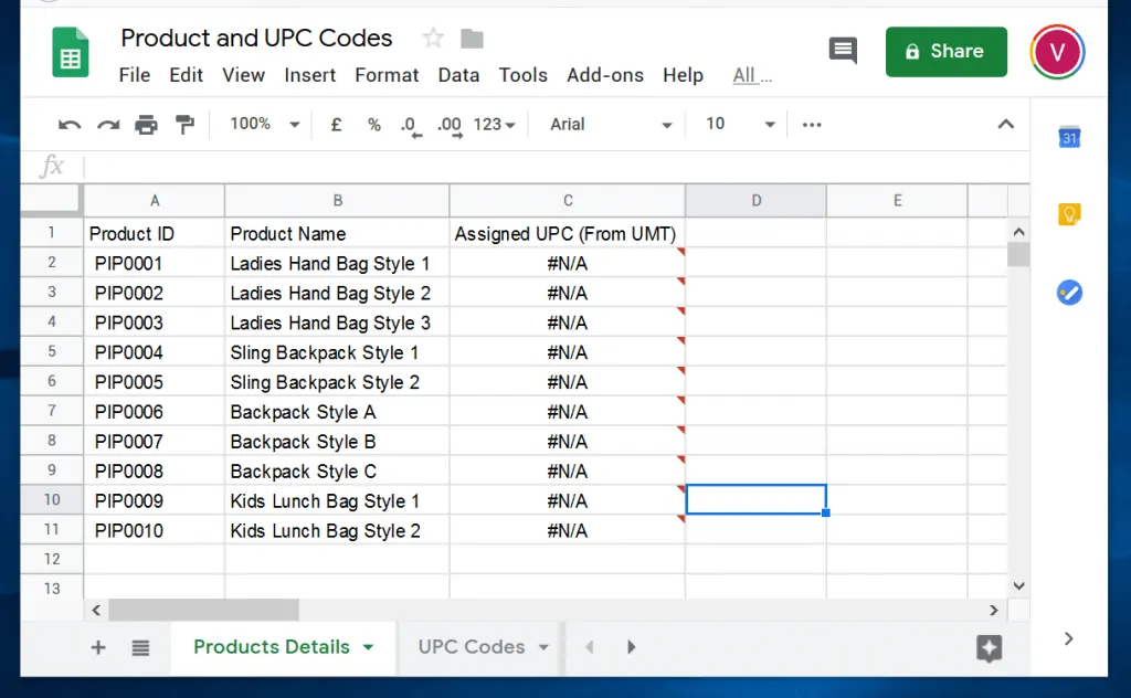
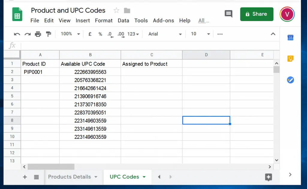
What the tool Does

If I enter a product ID from the Product Details worksheet into the Product ID column in the UPC Codes worksheet, VLOOPUP will automatically assign a UPC code to the product.

Here is the formula I used:

 =VLOOKUP(A2,'UPC Codes'!A2:B8,2,FALSE)

Here is the formula in Google Sheets.

VLOOKUP in Google Sheets Example Explained

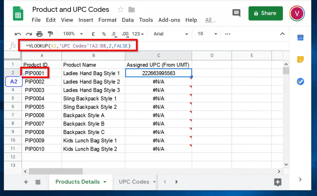
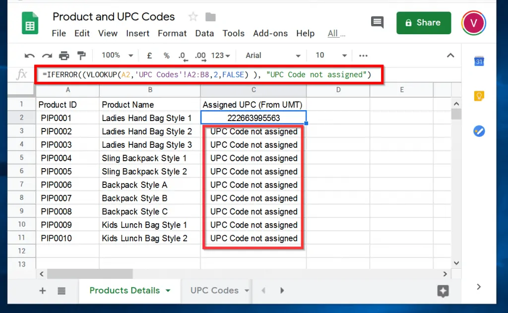
Refer to the last 2 images above. The first image shows the VLOOKUP formula in the Product Details worksheet. For reference, here is the formula.

=VLOOKUP(A2,'UPC Codes'!A2:B8,2,FALSE)

A2 contains the search_key – the look up value.

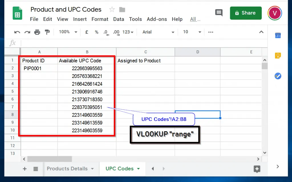
‘UPC Codes’!A2:B8 is the range that VLOOKUP will search for the search_key.

2 is index – this is the column that VLOOKUP will return from the range if it finds the search_key.

FALSE is the is_sorted value – indicates that the range is not sorted.

Here is how the formula works:

To assign the UPC code, 222663995563 to the product, I simply copy the product ID PIP0001 to cell A2 in the UPC codes worksheet. When VLOOKUP searches the range, A2:B8 in the UPC Codes worksheet, it finds the search_key. In this example, the search_key is the product ID PIP0001. It then returns the value in cell B2, the index column.

How to Resolve VLOOKUP in Google Sheets “#N/A” Error

In the above example, you would have noticed that if VLOOKUP does not find a match, it returns “#N/A” error. To remove this error and add some text, use the IFERROR function.

The Syntax of the IFERROR function is

IFERROR(value, [value_if_error])

value: this is the actual result that the VLOOKUP returns if there is no error. That is, if it finds the search_key in the specified range. However, if VLOOKUP returns an error IFERROR will return [value_if_error].

So, to resolve the “#N/A” error, replace value in IFERROR formula with the VLOOKUP formula shown below:

VLOOKUP(A2,'UPC Codes'!A2:B8,2,FALSE) 

The IFERROR formula will then look like this:

=IFERROR((VLOOKUP(A2,'UPC Codes'!A2:B8,2,FALSE) ), [value_if_error])

Next, replace [value_if_error] with a text like “UPC Code not assigned”

The IFERROR formula will now look like this:

=IFERROR((VLOOKUP(A2,'UPC Codes'!A2:B8,2,FALSE) ), "UPC Code not assigned")

Independent reader supportYour contribution helps us test, update, and keep practical guides available for everyone.Support on Ko-Fi

Conclusion

VLOOKUP in Google Sheets is an important function that you can use to solve many business problems. I hope this guide simplifies how to use VLOOKUP in Google Sheets.

I hope you found this guide helpful. If you did, let us know by sparing 2 minutes to share your experience with our community at [discourse_topic_url].

Furthermore, in the rare chance that you found it difficult to follow the steps in the guide or you followed the steps, but got stuck, please reply to this article’s topic at [discourse_topic_url]. Our team and other community members will come back to you with an answer as soon as possible.

Other Helpful Guides

• How to Make a Line Graph in Google Sheets
• How to Make a Line Graph in Excel

Additional Resources and References

• VLOOKUP
• VLOOKUP function
• [discourse_topic_url]

Product prices and availability are accurate as of the date/time indicated and are subject to change. Any price and availability information displayed on Amazon at the time of purchase will apply.